The interquartile range (IQR) identifies and eliminates the deviations from both ends of a data series. It also measures variation in cases of skewed data distribution. But, when we compare it with the standard deviation, it is less sensitive to extreme observations or values. For calculating the interquartile range, firstly, we need to calculate the Quartiles. Let us study the interquartile range formula in detail.
What are Quartiles?
The Quartiles divide a set of data series into four equal parts. The four parts are namely, First Quartile (Q1), Second Quartile (Q2), Third Quartile (Q3), and Fourth Quartile (Q4). We also know Second Quartile (Q2) as the Median of the data series as it also divides the data into two equal parts.
- First quartile: It divides the data such that one-fourth or the 25% of the values are below it and the remaining three-fourth or 75% are above it. We also call the first quartile as a lower quartile. We denote it as Q1.
- Second quartile: It divides the data or observations into two equal parts so that 50% of the observations are below it and 50% of the observations are above it. We also know it as Median. We denote it as Q2.
- Third quartile: It divides the series such that three-fourth or 75% of the observation is below it and the remaining one-fourth or 25% of the observations are above it. We also call the third quartile as the upper quartile. We denote it as Q3.
What is the Interquartile Range?
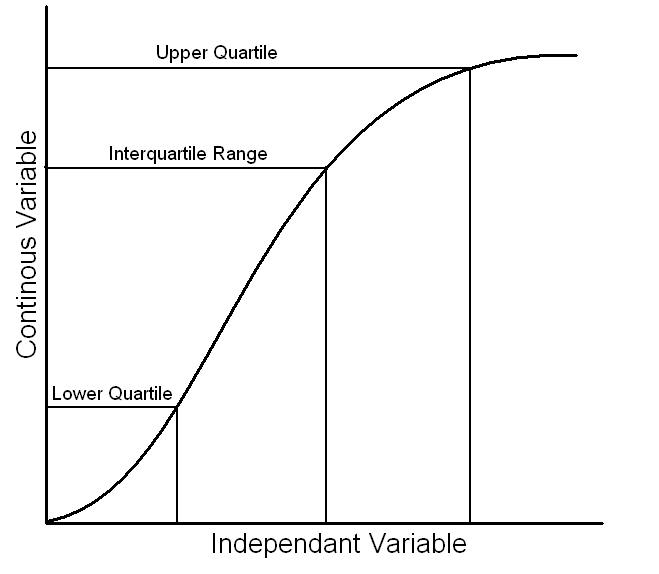
The interquartile range is a measure of variance. It represents the range from the 25th percentile to the 75th percentile. In other words, we can say that it represents the middle 50 percent of a data series. It is useful in determining the average range of observations. It is a more effective tool of analyzing the data in comparison to mean or median as it identifies the dispersion range.
Formula for Quartiles
1.Individual series
We need to arrange the values in ascending order, before calculating the quartiles.
- \(Q_1 = \frac{(N + 1)}{4}^th term\)
- \(Q_2 = \frac{(N + 1)}{2} term\)
- \(Q_3 = 3 \times \frac{(N + 1)}{4} term\)
Where, N is the number of observations
2. Discrete series
- \(Q_1 = \frac{(N + 1)}{4} term\)
- \(Q_2= \frac{(N + 1)}{2} term\)
- \(Q_3 = 3 \times \frac{(N + 1)}{4} term\)
Note: In discrete series, we need to calculate the cumulative frequency first. Then, we apply the formula. Then we see that the value that we get falls in which cumulative frequency. The observation corresponding to that cumulative frequency is our answer.
3. Continuous series
- \(Q_1 = l + \frac{\frac{N}{4} – c.f.}{f} \times h\)
- \(Q_3 = l + \frac{\frac{3N}{4} – c.f.}{f} \times h\)
| l | Lower limit of the quartile class interval |
| N | No. of observations |
| c.f. | Cumulative frequency of the preceding class |
| f | Frequency of the quartile class |
| h | Upper limit – the lower limit of the quartile class |
Note: For calculating the quartile class, apply the formula given under the individual series. If the answer is in fraction then round it off to integer.
Formula for Interquartile Range
And from the above equations, let us see the interquartile range formula
IQR = Q3 – Q1
| IQR | Interquartile range |
| Q3 | Third quartile |
| Q1 | First quartile |
Solved Examples for Interquartile Range Formula
Q.1: Find the inter-quartile range for the following data: 56, 14, 84, 21, 85, 2, 35, 74, 66, 52, 45
Solution: Arranging the data in ascending order: 2, 14, 21, 35, 45, 52, 56, 66, 74, 84, 85,
\(Q_1 = \frac{(N + 1)}{4} term\)
=\( \frac{11 + 1}{4} term\)
= 3rd term
= 21
And, \(Q_3 = 3 \times \frac{(N + 1)}{4} term\)
\(= 3 \times \frac{11 + 1}{4} term\)
\(= 3 \times 3 term\)
= 9th term
= 74
Interquartile Range = Q3 – Q1= 74 – 21 = 53


I get a different answer for first example.
I got Q1 as 20.5
median 23 and
Q3 26