Indifference Curve

A popular alternative to the marginal utility analysis of demand is the Indifference Curve Analysis. This is based on consumer preference and believes that we cannot quantitatively measure human satisfaction in monetary terms. This approach assigns an order to consumer preferences rather than measure them in terms of money. Let us take a look.

Browse more Topics under Theory Of Consumer Behavior

• Nature and Classification of Human Wants
• Marginal Utility Analysis
• Consumer Surplus
• Consumers Equilibrium

What is an Indifference Curve?

An indifference curve is a curve that represents all the combinations of goods that give the same satisfaction to the consumer. Since all the combinations give the same amount of satisfaction, the consumer prefers them equally. Hence the name indifference curve.

Here is an example to understand the indifference curve better. Peter has 1 unit of food and 12 units of clothing. Now, we ask Peter how many units of clothing is he willing to give up in exchange for an additional unit of food so that his level of satisfaction remains unchanged.

Peter agrees to give up 6 units of clothing for an additional unit of food. Hence, we have two combinations of food and clothing giving equal satisfaction to Peter as follows:

1. 1 unit of food and 12 units of clothing
2. 2 units of food and 6 units of clothing

By asking him similar questions, we get various combinations as follows:

Combination	Food	Clothing
A	1	12
B	2	6
C	3	4
D	4	3

Graphical Representation:

The diagram shows an Indifference curve (IC). Any combination lying on this curve gives the same level of consumer satisfaction. Another name for it is Iso-Utility Curve.

Indifference Map

An Indifference Map is a set of Indifference Curves. It depicts the complete picture of a consumer’s preferences. The following diagram shows an indifference map consisting of three curves:

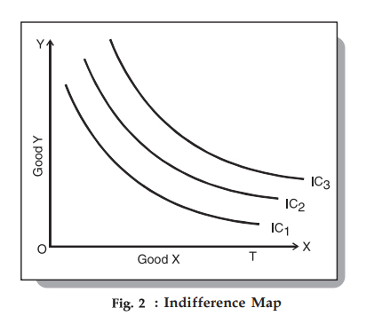
We know that a consumer is indifferent among the combinations lying on the same indifference curve. However, it is important to note that he prefers the combinations on the higher indifference curves to those on the lower ones.

This is because a higher indifference curve implies a higher level of satisfaction. Therefore, all combinations on IC1 offer the same satisfaction, but all combinations on IC2 give greater satisfaction than those on IC1.

Marginal Rate of Substitution

This is the rate at which a consumer is prepared to exchange a good X for Y. If we go back to Peter’s example above, we have the following table:

Combination	Food	Clothing	MRS
A	1	12	–
B	2	6	6
C	3	4	2
D	4	3	1

In this example, Peter initially gives up 6 units of clothing to get an extra unit of food. Hence, the MRS is 6. Similarly, for subsequent exchanges, the MRS is 2 and 1 respectively. Therefore, the MRS of X for Y is the amount of Y whose loss can be compensated by a unit gain of X, keeping the satisfaction the same.

Interestingly, as Peter accumulates more units of food, the MRS starts falling – meaning he is prepared to give up fewer units of clothing for food. There are two reasons for this:

1. As Peter gets more units of food, his intensity of desire for additional units of food decreases.
2. Most of the goods are imperfect substitutes for one another. If they could substitute one another perfectly, then MRS would remain constant.

Properties of an Indifference Curve or IC

Here are the properties of an indifference curve:

An IC slopes downwards to the right

This slope signifies that when the quantity of one commodity in combination is increased, the amount of the other commodity reduces. This is essential for the level of satisfaction to remain the same on an indifference curve.

An IC is always convex to the origin

From our discussion above, we understand that as Peter substitutes clothing for food, he is willing to part with less and less clothing. This is the diminishing marginal rate of substitution. The rate gives a convex shape to the indifference curve. However, there are two extreme scenarios:

1. Two commodities are perfect substitutes for each other – In this case, the indifference curve is a straight line, where MRS is constant.
2. Two goods are perfect complementary goods – An example of such goods would be gasoline and water in a car. In such cases, the IC will be L-shaped and convex to the origin.

Indifference curves never intersect each other

Two ICs will never intersect each other. Also, they need not be parallel to each other either. Look at the following diagram:

Fig 3 shows two ICs intersecting each other at point A. Since points A and B lie on IC1, they give the same satisfaction level to an individual. Similarly, points A and C give the same satisfaction level, as they lie on IC2. Therefore, we can imply that B and C offer the same level of satisfaction, which is logically absurd. Hence, no two ICs can touch or intersect each other.

A higher IC indicates a higher level of satisfaction as compared to a lower IC

A higher IC means that a consumer prefers more goods than not.

An IC does not touch the axis

This is not possible because of our assumption that a consumer considers different combinations of two commodities and wants both of them. If the curve touches either of the axes, then it means that he is satisfied with only one commodity and does not want the other, which is contrary to our assumption.

Indifference Curve Analysis

 Indifference curves are based on a number of assumptions, such as that each indifference curve is convex to the origin and that no two indifference curves ever overlap. When obtaining bundles of commodities on indifference curves that are farther from the origin, consumers are supposed to be more satisfied.

The majority of the time, indifference curve analysis assumes that all other variables are stable or constant.

The slope of the indifference curve is referred to by the MRS. The MRS measures how eager a consumer is to trade one product for another. If a customer values a banana, for example, the rate of substitution for watermelon will be slower, and the slope will reflect this rate of substitution.

Criticisms and Complications of the Indifference Curve

 Many components of current economics, like indifference curves, have been criticised for oversimplifying or making unreasonable assumptions about human behaviour. Consumer tastes, for example, might change dramatically over time, rendering accurate indifference curves useless.

Others argue that concave indifference curves, as well as circular curves that are convex or concave to the origin at specific points, are theoretically possible. Consumer preferences can change substantially over time, making accurate indifference curves obsolete.

Marginal Rate of Substitution

This is the rate at which a consumer is prepared to exchange a good X for Y. If we go back to Peter’s example above, we have the following table:

Combination	Food	Clothing	MRS
A	1	12	–
B	2	6	6
C	3	4	2
D	4	3	1

In this example, Peter initially gives up 6 units of clothing to get an extra unit of food. Hence, the MRS is 6. Similarly, for subsequent exchanges, the MRS is 2 and 1 respectively. Therefore, the MRS of X for Y is the amount of Y whose loss can be compensated by a unit gain of X, keeping the satisfaction the same.

Interestingly, as Peter accumulates more units of food, the MRS starts falling – meaning he is prepared to give up fewer units of clothing for food. There are two reasons for this:

1. As Peter gets more units of food, his intensity of desire for additional units of food decreases.

2. Most of the goods are imperfect substitutes for one another. If they could substitute one another perfectly, then MRS would remain constant.

Budget Line

Since a higher indifference curve represents a higher level of satisfaction, a consumer will try to reach the highest possible IC to maximize his satisfaction. In order to do so, he has to buy more goods and has to work under the following two constraints:

1. He has to pay the price for the goods and
2. He has limited income, restricting the availability of money for purchasing these goods

As can be seen above, a budget line shows all possible combinations of two goods that a consumer can buy within the funds available to him at the given prices of the goods. All combinations that are within his reach lie on the budget line.

A point outside the line (point H) represents a combination beyond the financial reach of the consumer. On the other hand, a point inside the line (point K) represents under-spending by the consumer.

Do you also want to know Consumers Equilibrium?

Solved Question on Indifference Curve

Q: What are the assumptions underlying the indifference curve approach?

Ans: The assumptions are as follows,

• The consumer is rational. Also, he possesses full information about all the relevant aspects of the economic environment in which he lives.
• The consumer can rank combination of goods based on the satisfaction they yield. However, he can’t quantitatively express how much he prefers a certain good over the other.
• If a consumer prefers A over B and B over C, then he prefers A over C.
• If a combination X has more commodities than the combination Y, then X is preferred over Y.